Classification and Decision Trees, Q4 2019

This course was given as part of the ML Boot Camp for Q4, 2019 and aims to introduce the audience to Classification. Additionally it allows the audience to work through different classification algorithms to understand the difference between them as well as get a feel for the implicit bias each algorithm has. The subsequent assignment allows them to practice their understanding on the subject.

Slides

• Classification
• Logistic Regression
• Decision Trees
• Evaluation Metrics

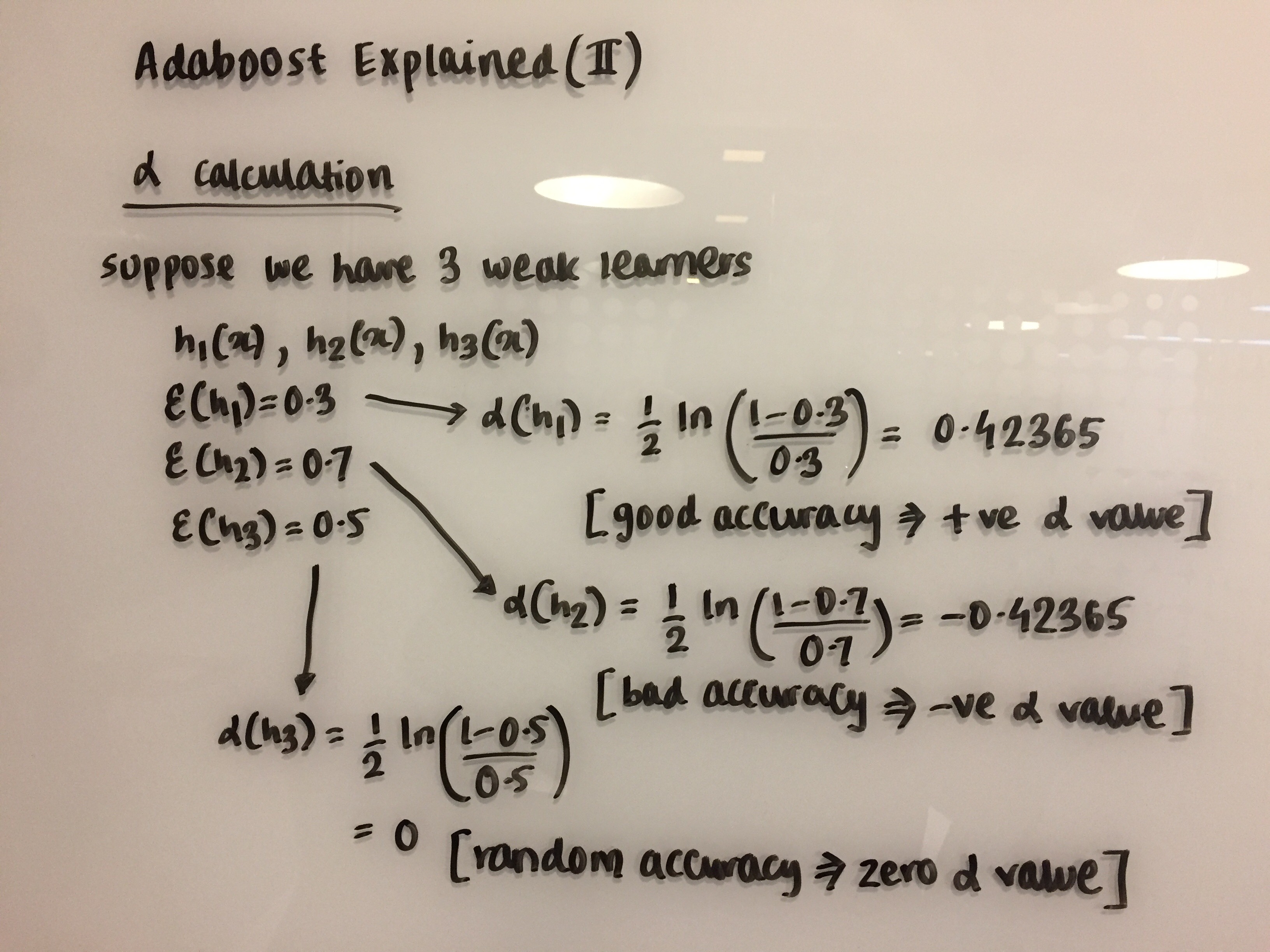
Adaboost explained

• Error computation
• Alpha computation
• Sample weight updation

Demos

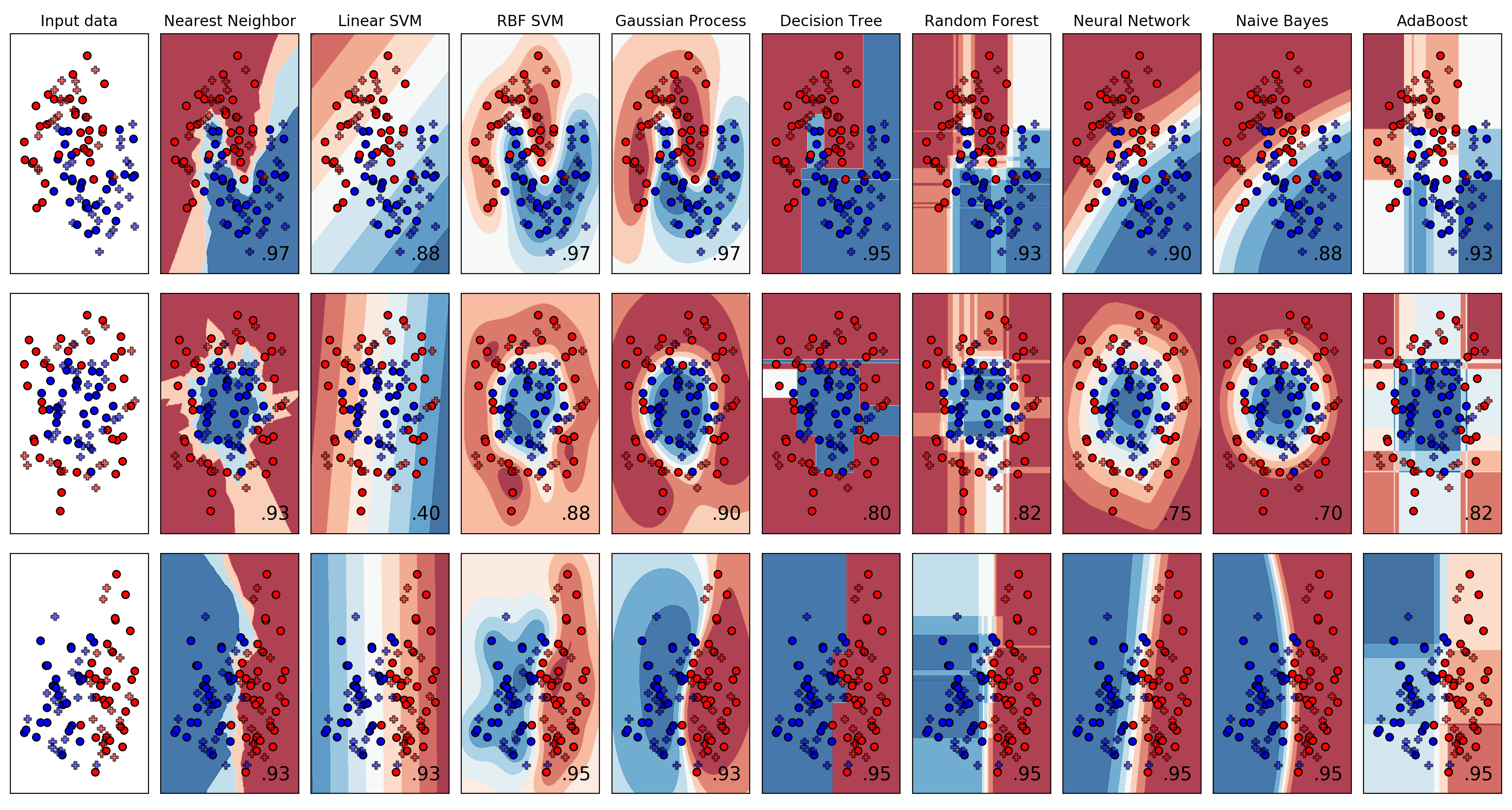
• Classifiers overview
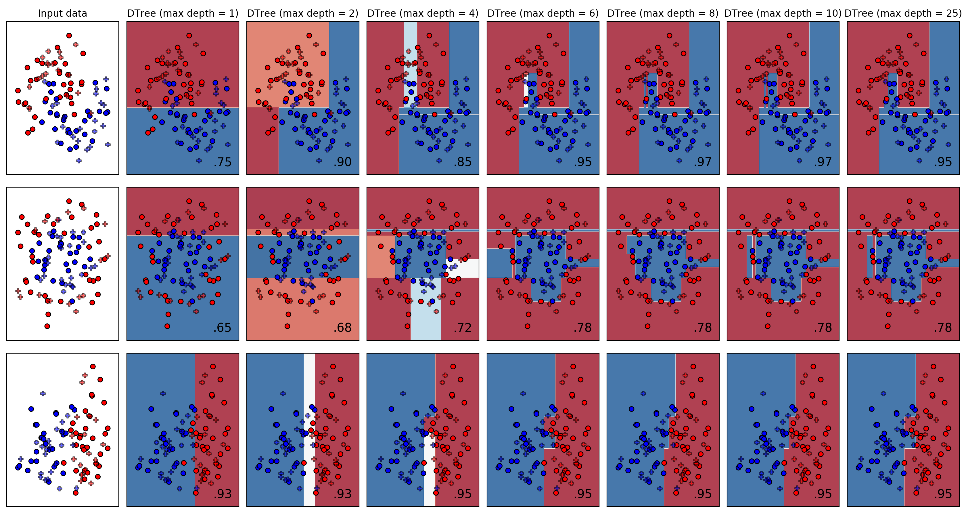
• Decision Tree based classification
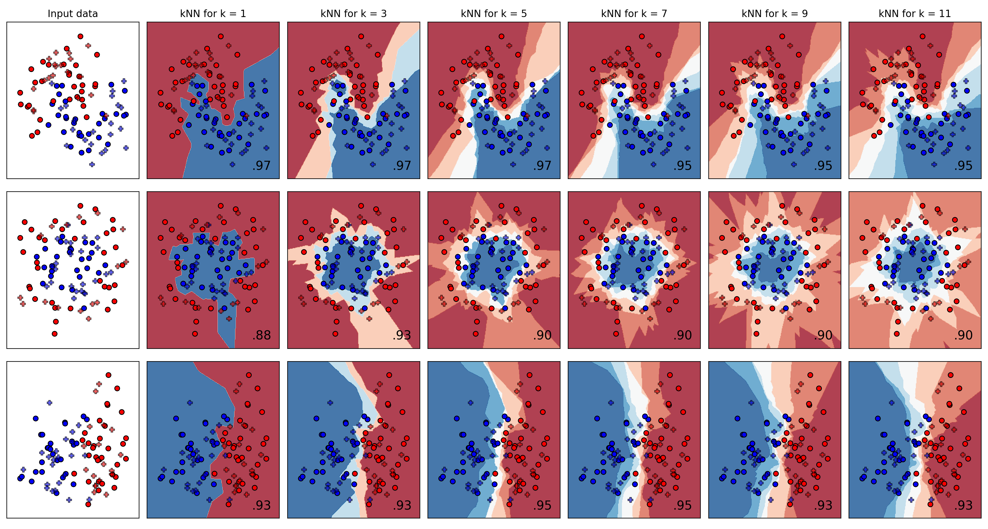
• Nearest Neighborhood based classification
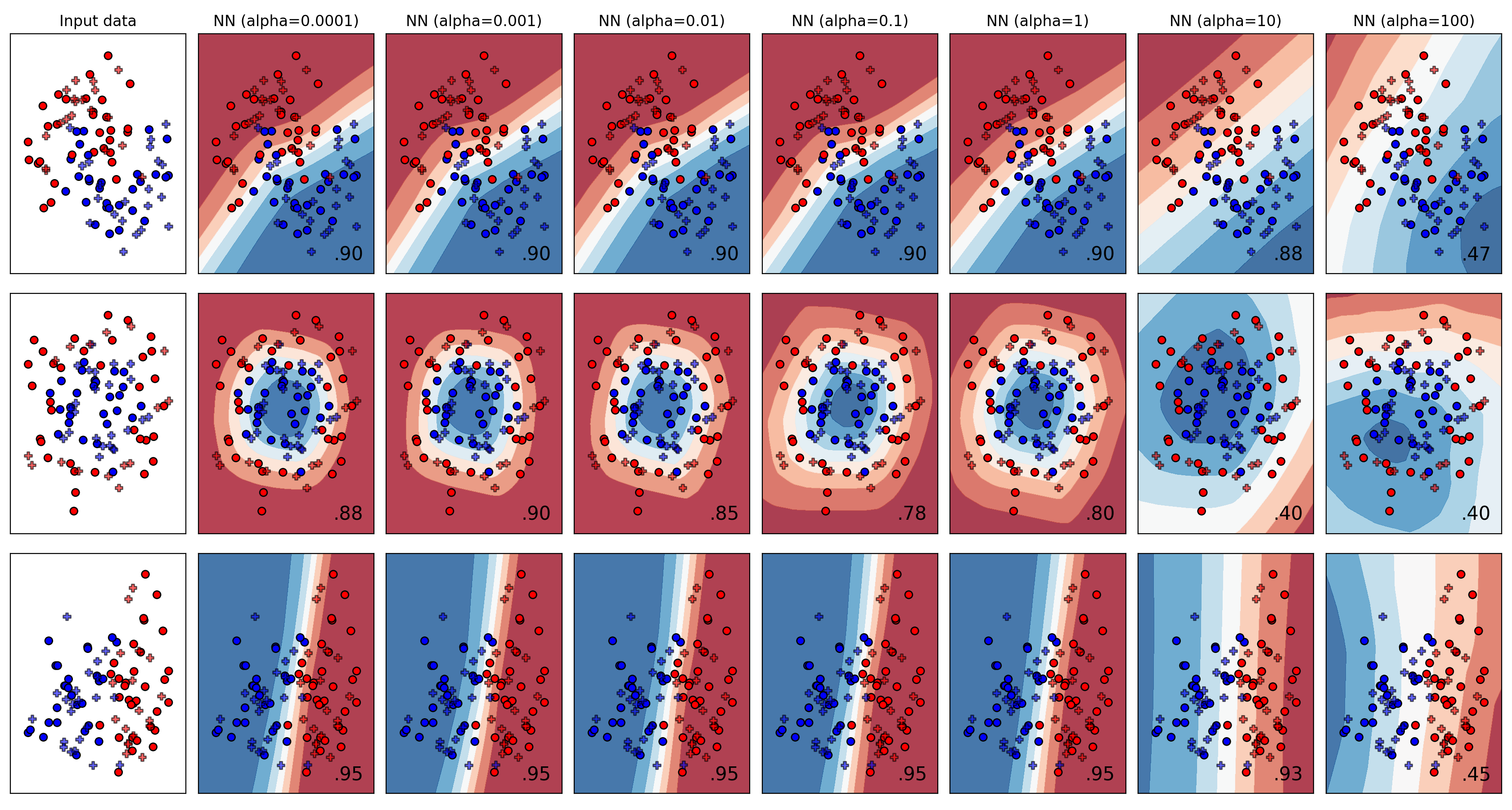
• Neural Network based classification
• Random Forest based classification
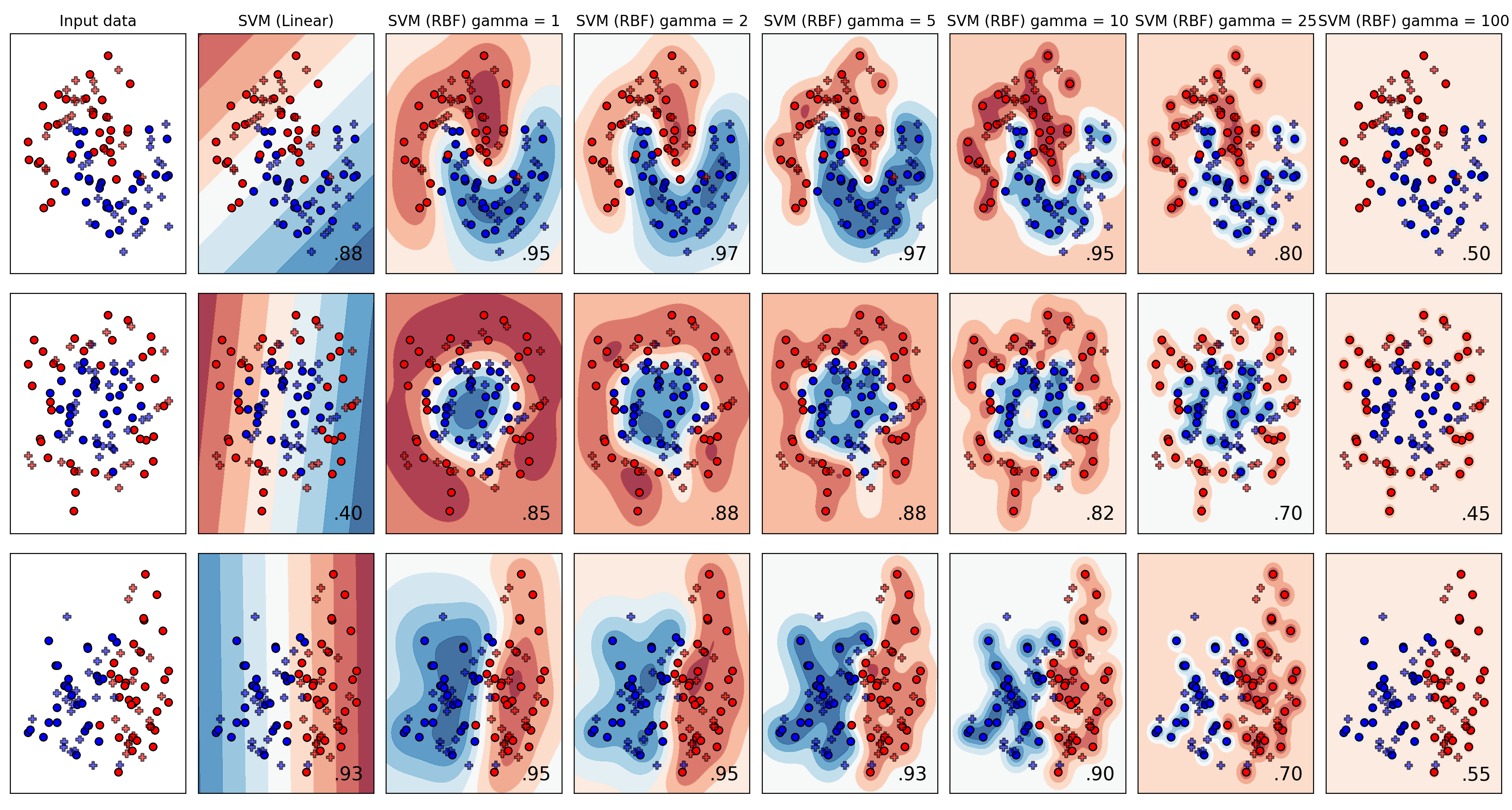
• SVM based classification
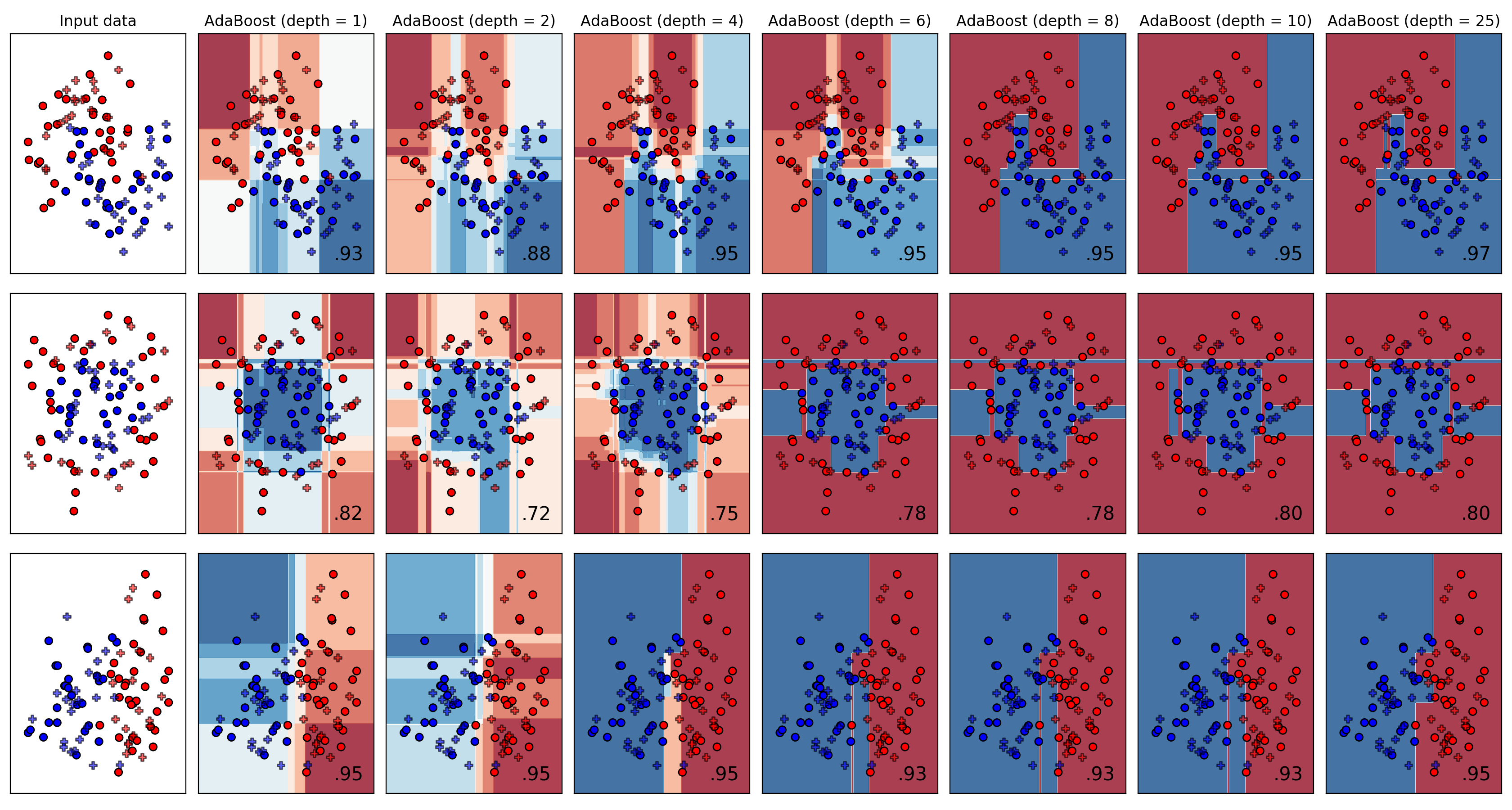
• Adaboost based classification

Assignment for the Machine Learning (ML) Bootcamp for Q4 2019 on “Classification and Decision Trees”

The best way to learn ML is to of course implement every algorithm from scratch. However I do not think we have the time and scope for the same, so I decided let us do the second best thing. Use a library for your assignment which has already implemented the algorithms and hence you can easily explore each of them and get a feel of what each algorithm tries to achieve.

Dataset

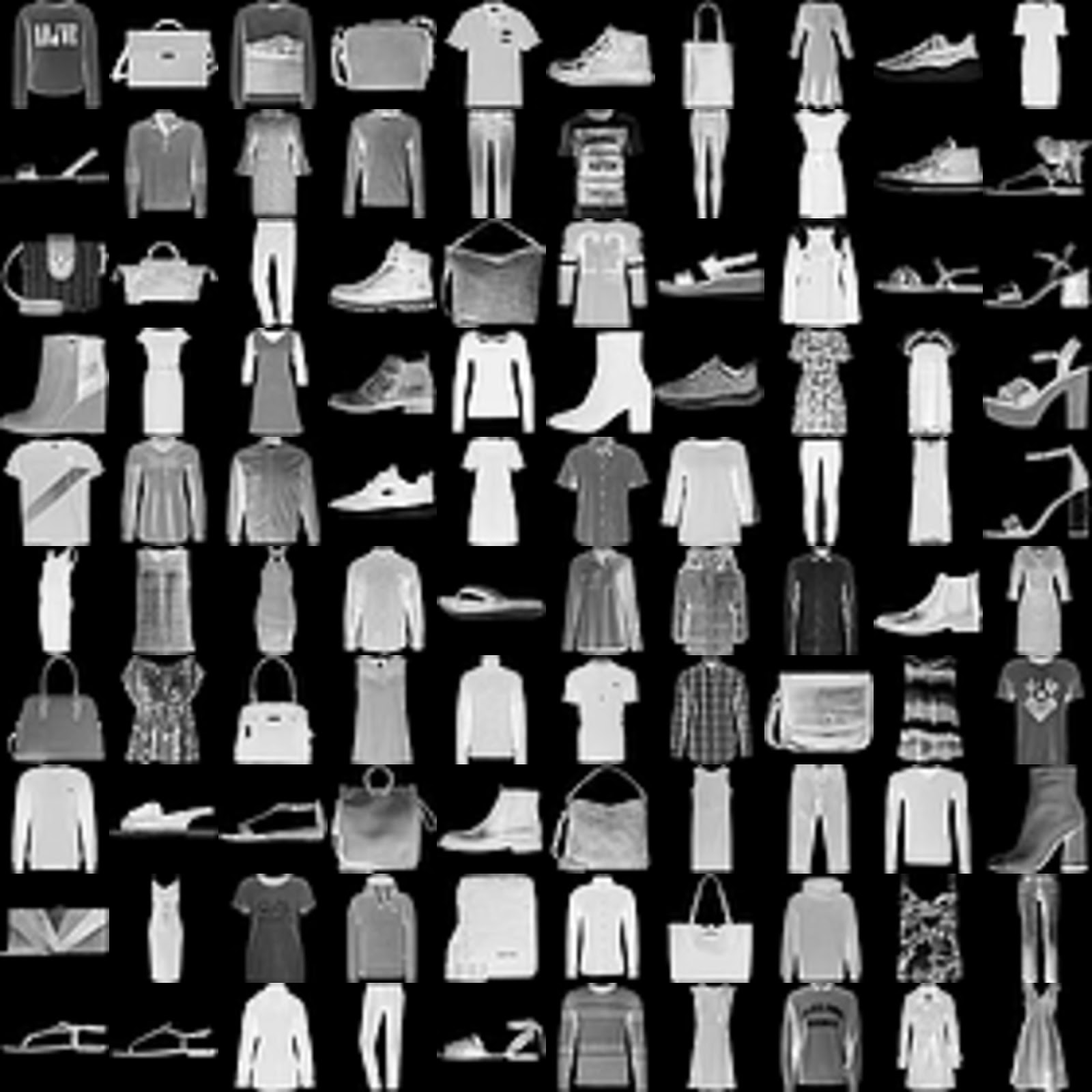
The dataset you will be using is the Fashion MNIST dataset. The reason for choosing this dataset is to make the assignment interesting. The prediction accuracies for the original MNIST dataset can be as high as 98% using even a simple 1-layer deep neural network (Ping me to know how in case you are interested! ). The dataset (both training and test data) can be found in the dataset sub-folder of this repository. See below to see how random samples from the Fashion MNIST dataset look like.

Algorithms to focus/explore on

• Nearest Neighborhood (NN) classification (k-Nearest Neighbors)
• Logistic Regression (LR)
• Decision Trees (DT)
• Random Forests (RF) (which are an ensemble of Decision Trees)
• Support Vector Machines (SVM) (linear as well as non-linear (using Radial Basis Functions))
• Multi-layer Perceptron (MLP)
• Adaboost (using DT classifiers as weak learners)

Coding

We will use Python for coding the assignment. The installation of Python on Mac is pretty simple and straightforward. Along with Python, you would require Numpy, Scipy and Matplotlib libraries. Please follow this simple tutorial for installation. Apart from this, you would require Scikit-learn. Scikit-learn is a ML library which is widely used and has pretty much all the ML algorithms implemented for end-users to use. Please follow tutorial for installing Scikit-learn.

Task

Explore the different classifiers listed above. Perform hyperparameter tuning for the different classifiers and observe its effect on test set accuracy -

• For NN, explore the effect of of varying the number of nearest neighbors
• For LR, explore the effect of varying inverse regularization coefficient parameter
• For DT, explore the effect of varying the max depth of the tree
• For RF, explore the effect of varying the number of trees in the forest as well as the maximum depth of each tree
• For SVM linear case, explore the effect of varying the penalty parameter
• For SVM non-linear case, explore the effect of varying the kernel multiplier parameter
• For MLP, explore the effect of varying the non-linear activation used as well as the L2 regularization coefficient parameter
• For Adaboost, explore the effect of varying the number of weak learners used as well as the learning rate parameter

Please explore at least 4-5 hyperparameter combinations for each of the classifiers (For LR, RF classifiers, please explore at least 8-10 hyperparameter combinations since there are two hyperparameters to vary together) above by varying the appropriate hyperparameter of the algorithm concerned.

Submission

Please submit a document which lists the different accuracy values you determined for each of the hyperparameter combinations you tried. Please also include your observations and any intuitions you had regarding why the effects of hyperparameter changes the result.

Please use hyperparameters in a reasonable range so that you can actually see its effect. Using very high or very low values might give you weird/unrepresentative to the truth results.

Tips and Tricks

• Try to normalize the data by dividing each of the (784 = 28-by-28) intensity values by 256 (which is the maximum pixel intensity). Normalizing the data usually results in better performance.
• Try to use Jupyter notebooks such that you would require to load the data only once in an earlier code block and can call different algorithms in later code blocks. Alternately you can write a script which can load the data first and subsequently vary your hyperparameters using a for loop construct. Feel free to use either.
• For the part of the assignment for SVM classifiers, it is a known fact that SVM classifiers typically do not scale well to large datasets i.e. time complexity to fit the SVM() classifier is proportional to square of the number of instances. The solution for this as mentioned here is to increase the kernel cache size i.e. call SVM() via setting the cache_size parameter to larger values as much as possible, for example SVM(C=1, cache_size=2000) or SVM(gamma=0.001, cache_size=2000) etc. Using cache_size=2000, SVM training finished in ~42.5 minutes, whereas using cache_size=4000, SVM training completed in ~41.65 minutes. Thus we can observe a law of diminishing returns. Also note that feature scaling also helps significantly thus it is strongly recommended to do the data normalization step mentioned above.
• Please feel free to use the code below to be able to plot/visualize the low-dimensional representations you get from each of the classifiers. The first function generates a 2-dimensional representation while the latter plots in 3 dimensions. I have also included options for visualing the plot as well as saving it. You can also plot one class at a time instead of plotting all classes at the same time using the for loop.

# X = test data which is a matrix of size 10000-by-784
# y = predicted labels i.e. the prediction using the classifier used, which is a vector of size 10000-by-1 
# labels_size = number of classes for your data (for Fashion MNIST for example = 10)

def display_2D(X, y, labels_size=10):
	import matplotlib
	import matplotlib.cm as cm
	import matplotlib.pyplot as plt
	from sklearn.decomposition import PCA

	fig = plt.figure(figsize=[20, 10])
	ax = plt.subplot(111)

	for label_idx in range(labels_size):
		indices = np.where(y == label_idx)[0]
		data = X[indices, :]
		data_lde = PCA(n_components = 2).fit_transform(data)

		plt.plot(data_lde[:, 0], data_lde[:, 1], marker='+', linewidth=0, label = 'Label = ' + str(label_idx))

	plt.xlabel('Latent Dimension #1')
	plt.ylabel('Latent Dimension #2')
	
	plt.title('Low-dimensional representation for Fashion-MNIST')
	plt.legend()

	ax.xaxis.set_tick_params(size=0)
	ax.yaxis.set_tick_params(size=0)

	xlab = ax.xaxis.get_label()
	ylab = ax.yaxis.get_label()

	xlab.set_style('italic')
	xlab.set_size(14)
	ylab.set_style('italic')
	ylab.set_size(14)

	ttl = ax.title
	ttl.set_weight('bold')

	#plt.show()
	fig.savefig('display_2D.png', bbox_inches='tight')

def display_3D(X, y, labels_size=10):
	import matplotlib
	import matplotlib.cm as cm
	import matplotlib.pyplot as plt
	from sklearn.decomposition import PCA
	from mpl_toolkits.mplot3d import Axes3D

	fig = plt.figure(figsize=[20, 10])
	ax = fig.add_subplot(111, projection='3d')

	for label_idx in range(labels_size):
		indices = np.where(y == label_idx)[0]
		data = X[indices, :]
		data_lde = PCA(n_components = 3).fit_transform(data)

		ax.scatter(data_lde[:, 0], data_lde[:, 1], data_lde[:, 2], marker='+', label = 'Label = ' + str(label_idx))

	ax.set_xlabel('Latent Dimension #1')
	ax.set_ylabel('Latent Dimension #2')
	ax.set_zlabel('Latent Dimension #3')
	
	plt.title('Low-dimensional representation for Fashion-MNIST')
	plt.legend()

	ax.xaxis.set_tick_params(size=0)
	ax.yaxis.set_tick_params(size=0)

	xlab = ax.xaxis.get_label()
	ylab = ax.yaxis.get_label()
	zlab = ax.zaxis.get_label()

	xlab.set_style('italic')
	xlab.set_size(14)

	ylab.set_style('italic')
	ylab.set_size(14)

	zlab.set_style('italic')
	zlab.set_size(14)

	ttl = ax.title
	ttl.set_weight('bold')

	plt.show()
	#fig.savefig('display_3D.png', bbox_inches='tight')