
Generative Models, Q4 2019
class, ML Boot Camp, Criteo Research, 2019
This course was given as part of the ML Boot Camp for Q4, 2019 aims to introduce the audience to Generative Models. The core intuition of latent spaces and manifolds and generative modeling are introduced. The subsequent assignment based on interpolation in latent spaces allows them to practice their understanding on the subject.
Slides
Assignment for the Machine Learning (ML) Bootcamp for Q4 2019 on “Generative Models”
In this assignment, you will -
- Understand how generative models work i.e. how do they generate etc.
- Appreciate the importance for non-linear dimension reduction (NLDR) for everyday ML tasks.
To do this, we will be working with a standard NLDR technique i.e. the Autoencoder. We have already seen the limitations of linear dimension reduction (LDR) i.e. PCA during the lecture. Just so that you can focus completely on learning and understanding Autoencoders, I will provide you with all the code you will need (check the ‘code’ sub-folder of this repository and also see below). Every line of the code has detailed explanations so that you can play around with it.
For the assignment, you will interpolate in between the latent spaces for MNIST digits. Firstly, because it is really cool to do so. Secondly, as you will get an intuition for latent spaces and manifolds.
Dataset
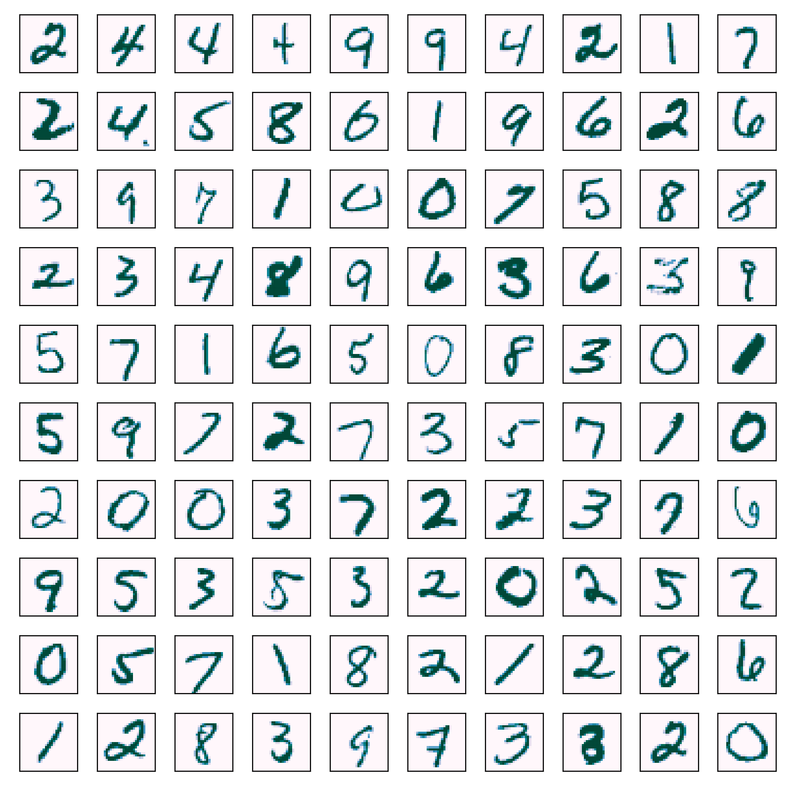
The dataset you will be using is the MNIST dataset. The MNIST dataset consists of images of handwritten digits for the numbers 0-9. It has 60000 training instances and 10000 test instances. The dataset (both training and test data sets) are available in the ‘data’ sub-folder of this repository. See below to see how random samples from the MNIST dataset look like.
Installation
The assignment needs to be completed using Python (Tensorflow and other libraries). The installation of Python on Mac is pretty simple and straightforward. Please follow the instructions below for installing Tensorflow and other requisite libraries. The course repository contains a miniconda installer and a requirements text file in the ‘installer’ sub-folder of this repository. Please download both to a local folder on your laptop before starting the assignment.
# 1) download the miniconda installer + requirements file from the course repository into a local folder on your laptop
# 1a) [optional] you can also try to download from https://docs.conda.io/en/latest/miniconda.html in case your OS is not MacOSX.
# 2) add/modify necessary permissions for miniconda installer
chmod +x Miniconda3-latest-MacOSX-x86_64.sh

# 3) install miniconda locally into your home and update your ~/.bashrc (i.e. accept all the modifications proposed)
./Miniconda3-latest-MacOSX-x86_64.sh

# 4) reload your bash
source ~/.bashrc

# 5) create environment tf_env
conda create -y --name tf_env python=3.6

# 6) activate environment
source activate tf_env

# please note that you need to execute all your python code for this assignment inside this miniconda environment by activating the environment
# to deactivate an miniconda environment, use the command -> 'source deactivate'

# 7) install dependencies including TF and Jupyter
pip install --upgrade -r requirements.txt

# 8) make sure everything is working fine using this simple test
python -c 'import tensorflow as tf; print(tf.__version__)'
Here are the contents of the file requirements.txt.
# Basic packages needed for the assignment on "Generative Models"

numpy
scipy
jupyter
matplotlib
scikit-learn

################################################################
# We are going to use the CPU version of Tensorflow for the assignment

tensorflow      # CPU Version of TensorFlow.
Task
For this assignment, we will be using neural networks and train Autoencoder models of different configurations for MNIST data. The training will be done using Batch Stochastic Gradient Descent. There are three different neural network settings you will explore which are as follows.
setting 1 - (To use this, please replace lines 95-97 in ‘tf_ae_mnist.py’ with the below snippet)
D1 = 128
D2 = 64
D3 = 2
setting 2 - (To use this, please replace lines 95-97 in ‘tf_ae_mnist.py’ with the below snippet)
D1 = 512
D2 = 128
D3 = 16
setting 3 - (To use this, please replace lines 95-97 in ‘tf_ae_mnist.py’ with the below snippet)
D1 = 1024
D2 = 128
D3 = 64
The task has three parts as follows :-
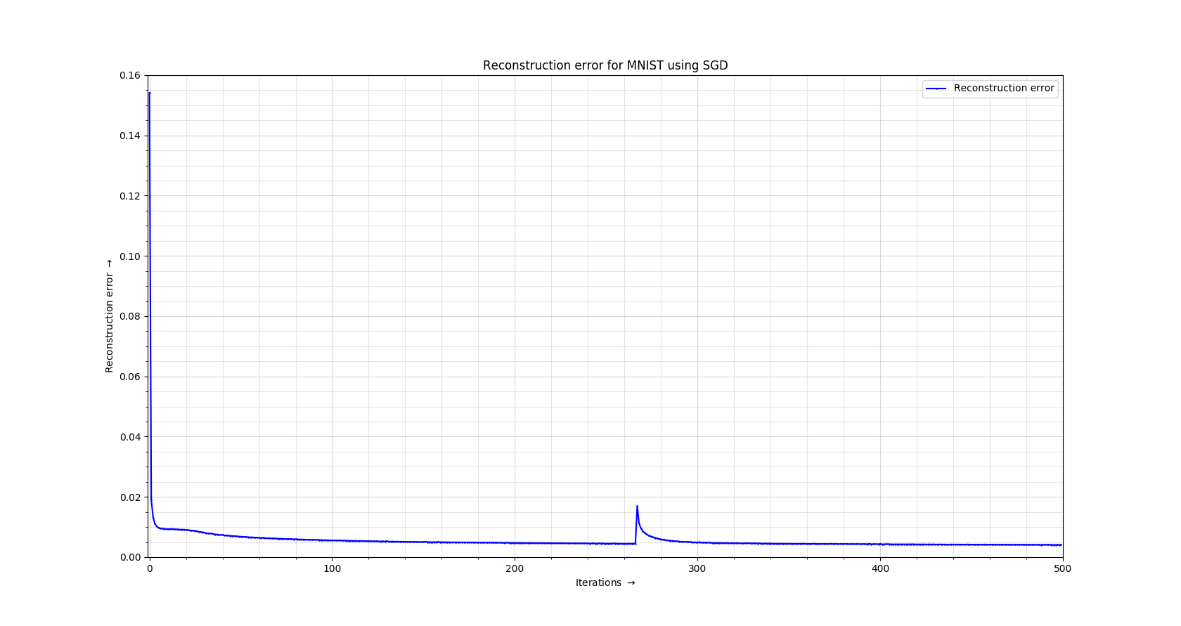
- In the first part, you will be studying the relationship between reconstruction error and the latent dimensionality of the embedding. To do this, you will run each of the different configurations and subsequently save and plot the reconstruction error for the three above network configurations. The provided code already does this. For example, this is how the recreation error curve looks like for some neural network setting.
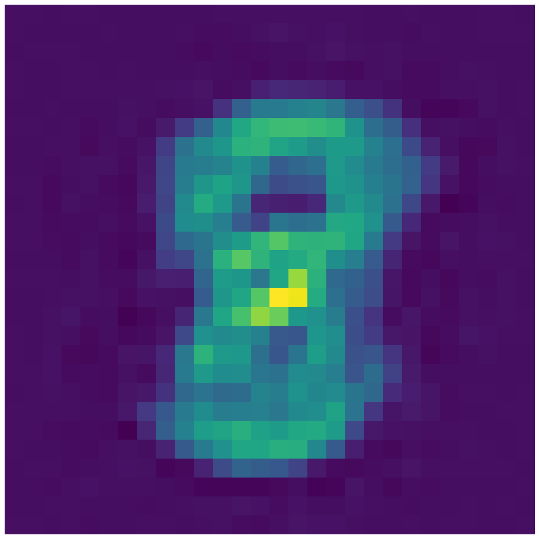
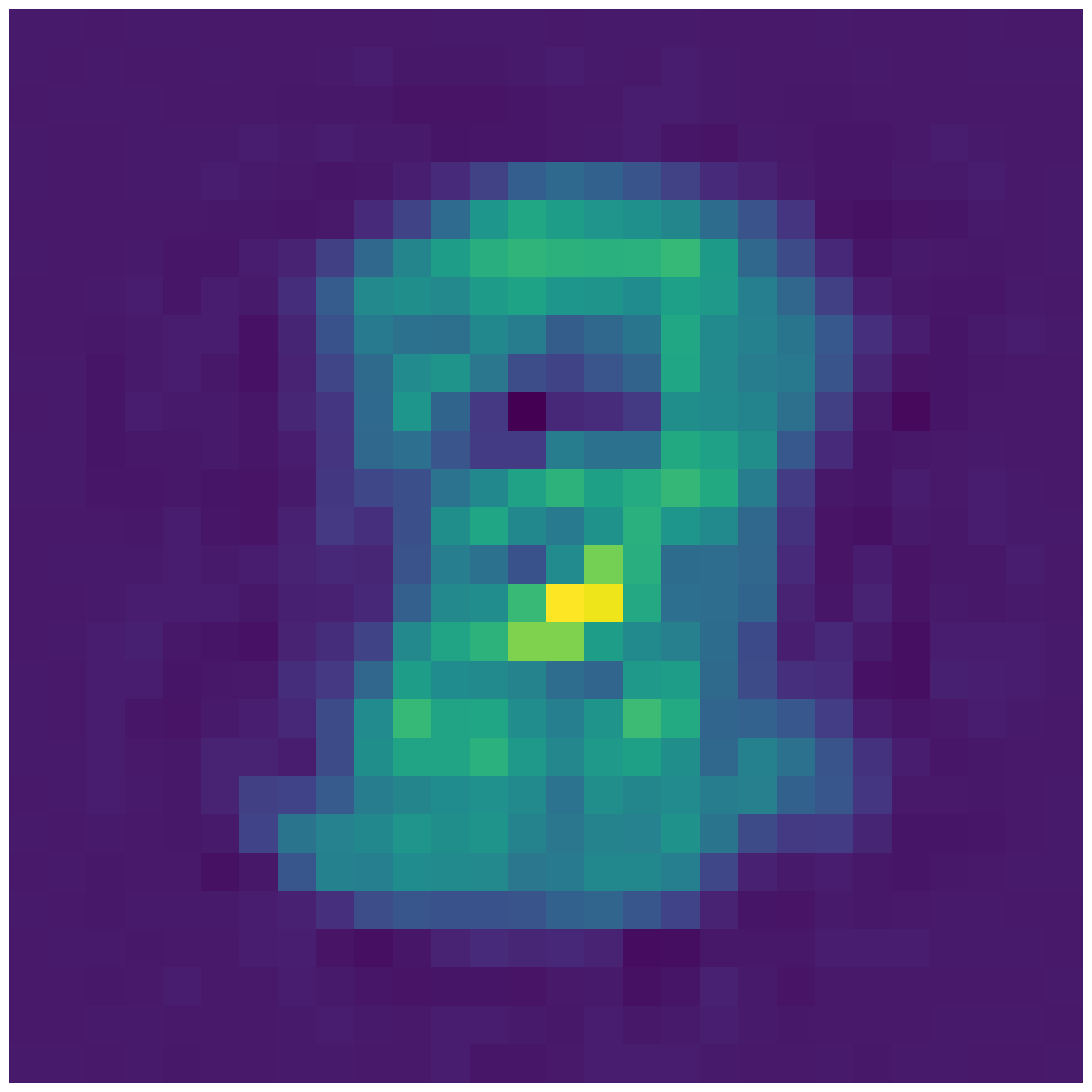
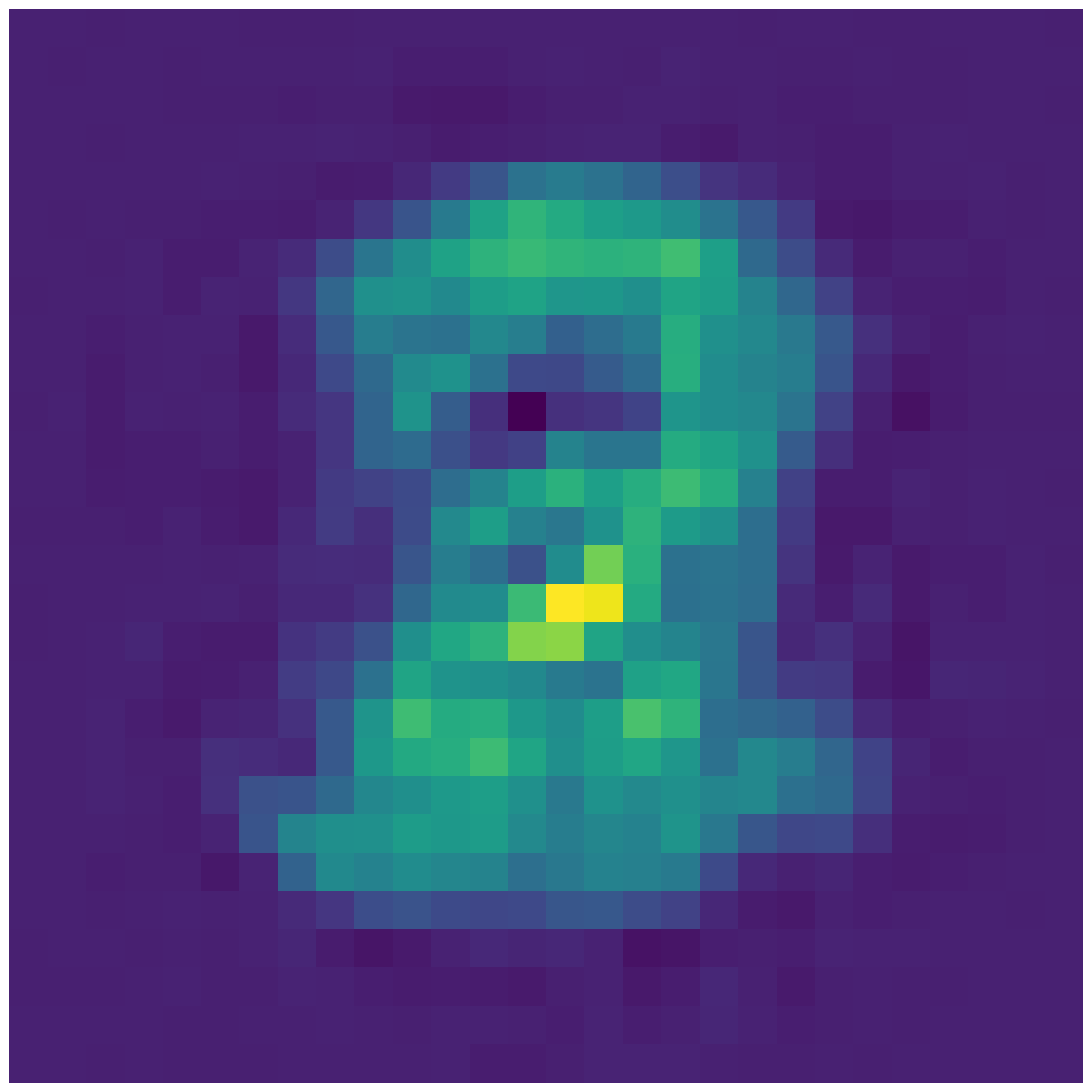
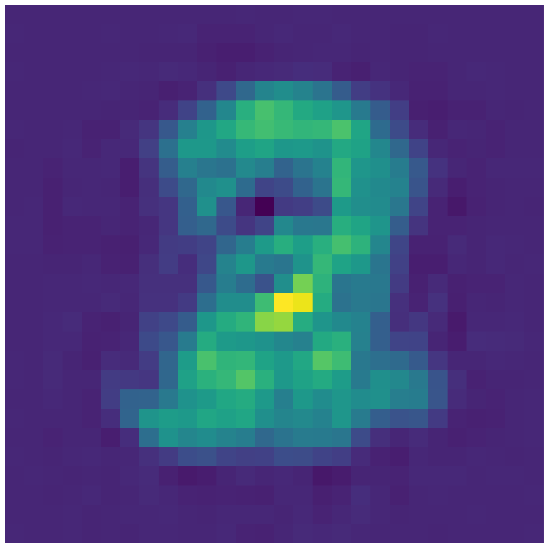
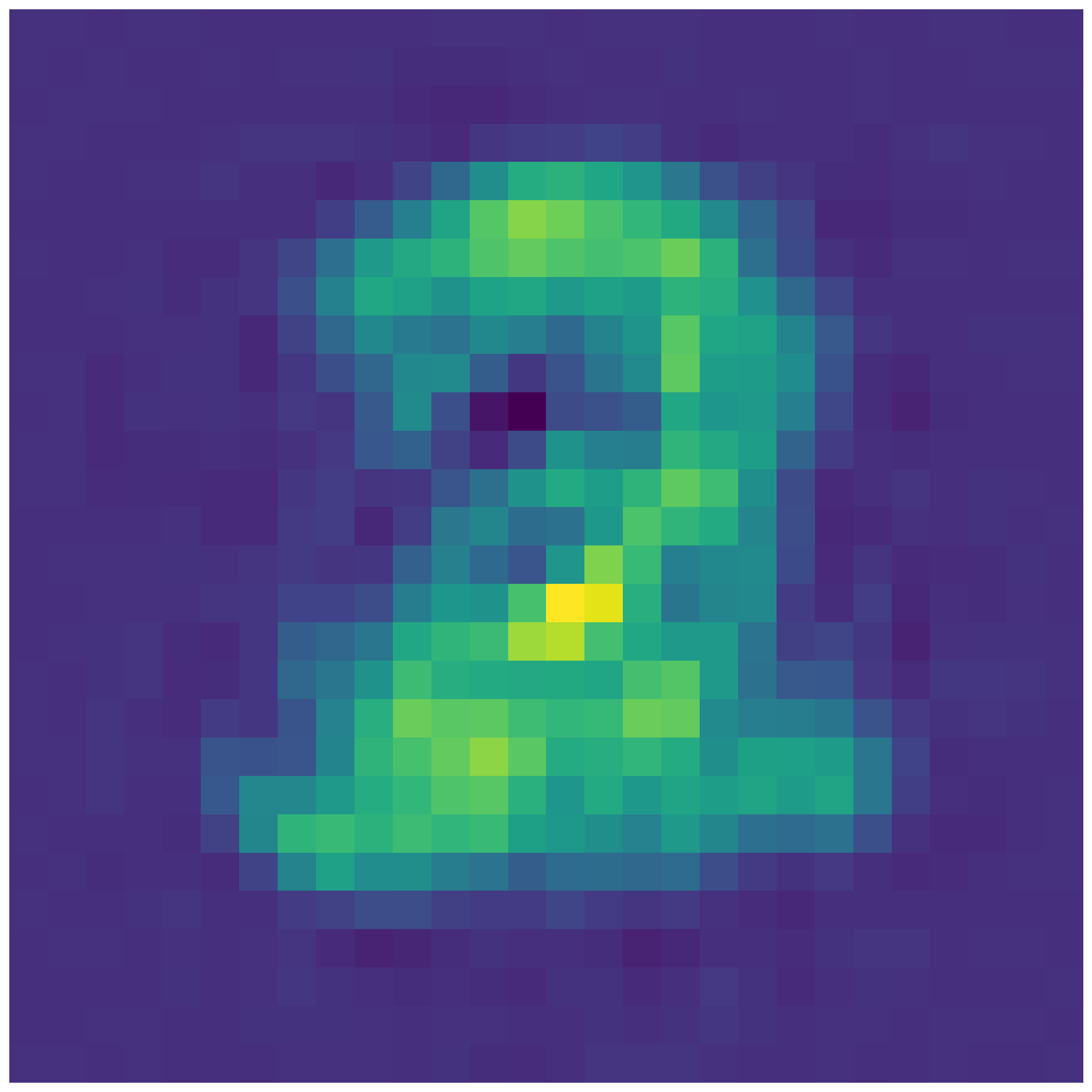
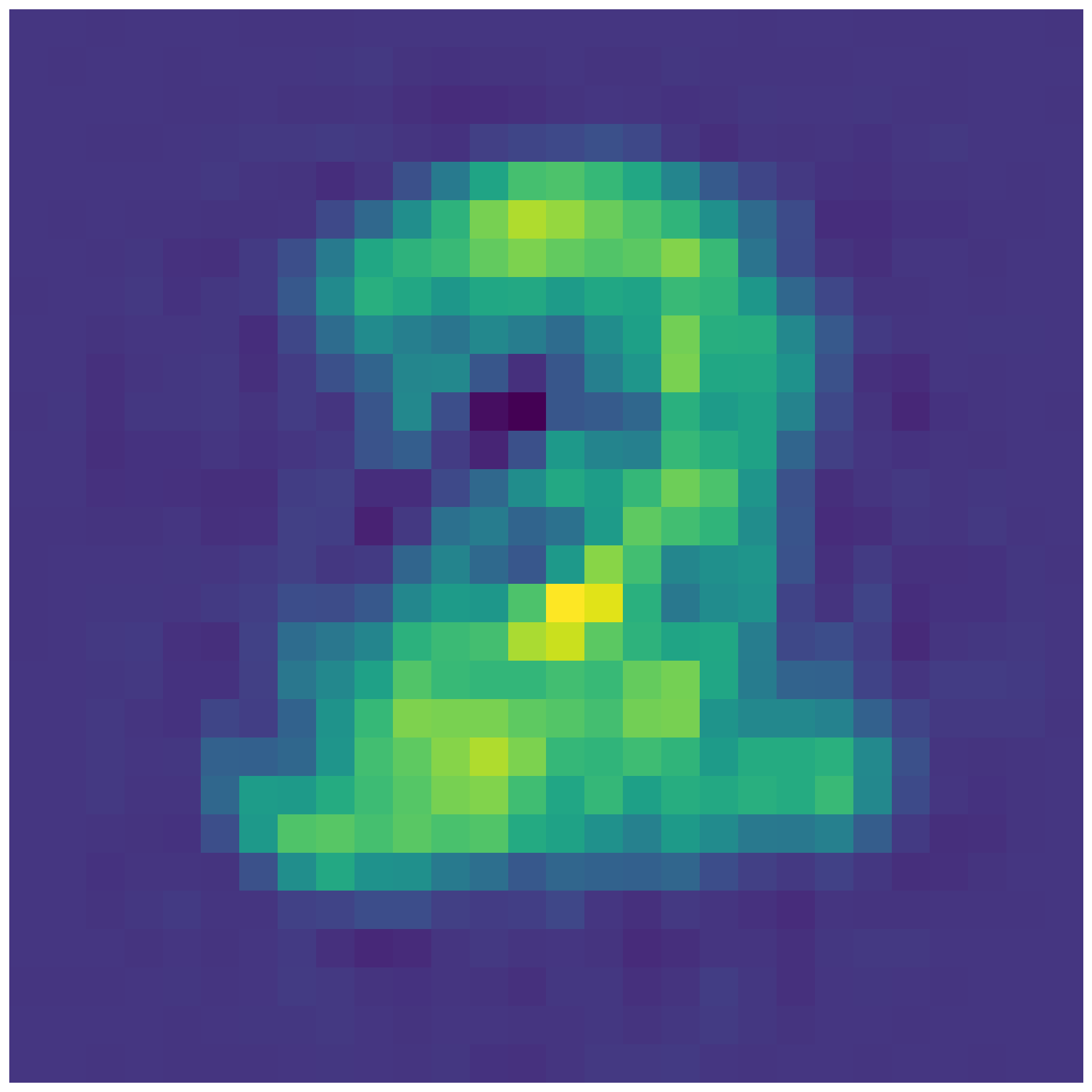
- In the second part, you will interpolate in latent spaces i.e. using the provided code to interpolate between the mean latent representation of different digits. See below for an example. Can you guess the two digits between which we are interpolating in latent space ? Please choose three different combinations of interpolations to be done using either setting 2 or 3. Please feel free to choose whatever digits you want to interpolate between. To do this part, please take a look at example 1 in ‘tf_ae_mnist.py’ and example 2 in ‘plot_lde.py’.


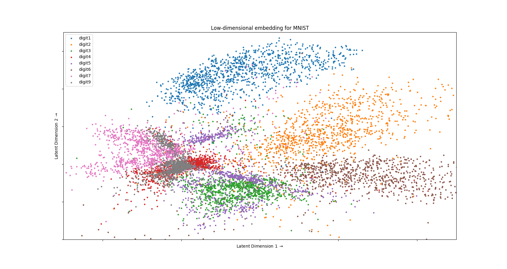
- In the third part, you will plot the 2-D embedding for the test dataset of MNIST (similar to what you saw in class). To do this part, please refer to example 3 in ‘plt_2d.py’.
Submission
Please submit a report/document which has all three parts included in it. Please also include your observations and any intuitions you have regarding the results you obtained.
Code
Here is the code in the main file ‘tf_ae_mnist.py’
from __future__ import absolute_import
from __future__ import division
from __future__ import print_function

import numpy as np
import tensorflow as tf

training_size = 60000 # number of training samples
test_size = 10000 # number of test samples
feature_size = 784 # feature size
class_size = 10 # number of classes in MNIST

nf = 255.0 # normalizing factor for features

lr = 0.001 # learning rate
iterations = 100000 # number of batch iterations for learning
batch_size = 500 # batch size
freq = 100 # frequency with which results are displayed or saved

# load training/test data and normalize begin

print('loading MNIST data')

train_data = np.loadtxt('', delimiter=',') # EDIT ME - add path for MNIST training data
test_data = np.loadtxt('', delimiter=',') # EDIT ME - add path for MNIST test data

print('loading MNIST data done')

x_train = np.asfarray(train_data[:, 1:]) / nf # normalizes training data
x_test = np.asfarray(test_data[:, 1:]) / nf # normalizes test data

y_train = np.asfarray(train_data[:, :1]) # extracts training labels
y_test = np.asfarray(test_data[:, :1]) # extracts test labels

# load training/test data and normalize end
# shuffle training/test data begin

shuffle_index = np.random.permutation(training_size) # creates permutation for random shuffling
x_train, y_train = x_train[shuffle_index, :], y_train[shuffle_index, 0] # shuffles data, labels

shuffle_index = np.random.permutation(test_size) # creates permutation for random shuffling
x_test, y_test = x_test[shuffle_index, :], y_test[shuffle_index, 0] # shuffles data, labels

print('data preprocessing done')

batch_idx = 0 # batch index to allow for dynamic batching of training data

# represents a single layer of dnn
def phi(x, n_output, name=None, activation=None, reuse=None):
    if len(x.get_shape()) != 2:
        x = flatten(x, reuse=reuse)

    n_input = x.get_shape().as_list()[1]

    with tf.variable_scope(name, reuse=reuse):
        W = tf.get_variable(
            name='W',
            shape=[n_input, n_output],
            dtype=tf.float32,
            initializer=tf.contrib.layers.xavier_initializer())

        b = tf.get_variable(
            name='b',
            shape=[n_output],
            dtype=tf.float32,
            initializer=tf.constant_initializer(0.0))

        h = tf.nn.bias_add(
            name='h',
            value=tf.matmul(x, W),
            bias=b)

        if activation:
            h = activation(h)

    return h, W

# generates next batch for training
def get_next_batch():
    global batch_idx # allow usage of global variable

    x_batch = np.zeros((batch_size, feature_size)) # temporary store for training batch data
    #y_batch = np.zeros((batch_size, class_size))

    for idx in range(batch_size): # gets batch data of size 'batch_size'
        x_batch[idx, :] = x_train[batch_idx, :] # copies from training data

        batch_idx += 1 # increment batch index

        if batch_idx == training_size: #reset batch index if it is equal to training size
            batch_idx = 0

    return x_batch

D1 = # EDIT ME - add width for first encoding/decoding layer
D2 = # EDIT ME - add width for second encoding/decoding layer
D3 = # EDIT ME - add width for third encoding/decoding layer

x = tf.placeholder(tf.float32, [None, feature_size]) # input layer

out_1, wt_1 = phi(x, D1, activation=tf.nn.tanh, name='encode_layer_1') # first encoding layer
out_2, wt_2 = phi(out_1, D2, activation=tf.nn.tanh, name='encode_layer_2') # second encoding layer
out_3, wt_3 = phi(out_2, D3, activation=None, name='latent_embedding_layer') # latent embedding layer
out_4, wt_4 = phi(out_3, D2, activation=tf.nn.tanh, name='decode_layer_1') # first decoding layer
out_5, wt_5 = phi(out_4, D1, activation=tf.nn.tanh, name='decode_layer_2') # second decoding layer

x_recreation, wt_6 = phi(out_5, feature_size, activation=None, name='output_layer') # output layer
loss_fn = tf.reduce_mean(tf.squared_difference(x, x_recreation)) # tensorflow object for loss function

train_step = tf.train.AdamOptimizer(learning_rate=lr).minimize(loss_fn) # tensorflow object for optimizer

sess = tf.Session() # starts a tf session

init_op = tf.global_variables_initializer() # initializes tf global variables
sess.run(init_op) # initializes tf global variables

print('starting model training')

errors = np.zeros((int(iterations/freq), 1)) # to keep track of reconstruction error over iterations

log_idx = 0 # log index to keep track of Minibatch Stochastic Gradient Descent

for idx in range(iterations):
    batch_xs = get_next_batch() # gets next stochastic minibatch

    sess.run(train_step, feed_dict={x: batch_xs}) # training single step

    if idx % freq == 0: # log reconstruction error every 100 iterations
        loss = sess.run(loss_fn, feed_dict={x: x_test}) # gets accuracy for current model
        errors[log_idx, :] = loss # register reconstruction loss

        log_idx += 1 # increment log index

        print(str(idx + 1) + '/' + str(iterations) + ': Reconstruction error = ' + str(loss)) # prints reconstruction error

embedding = sess.run(out_3, feed_dict={x: x_test}) # low-dimensional code or embedding computed

np.savetxt('recreation_err.csv', errors, delimiter=',') # saves recreation error over Minibatch Stochastic Gradient Descent iterations
np.savetxt('low_dimension_embedding.csv', embedding, delimiter=',') #EDIT ME - as needed to save the low-dimensional embedding for the MNIST test dataset
np.savetxt('mnist_test_labels.csv', y_test, delimiter=',') #EDIT ME - as needed to save the labels for the MNIST test dataset

# Example 1 - code to interpolate between the latent representation of 2 and 8

indices = np.where(y_test == 2) # indices of test dataset which contain instances for digit '2'
data2 = embedding[indices[0],:] # extracting all digit '2' instances
mean2 = np.mean(data2, 0) # compute 'mean' of all digit '2' instances to get average '2' latent representation

indices = np.where(y_test == 8) # indices of test dataset which contain instances for digit '8'
data8 = embedding[indices[0],:] # extracting all digit '8' instances
mean8 = np.mean(data8, 0) # compute 'mean' of all digit '8' instances to get average '8' latent representation

for frac_idx in range(11):
    f = float(frac_idx/10) # f iterates over values [0.0, 0.1, 0.2 ... 1.0]
    lde = np.zeros((1, D3)) # temporary variable to store low-dimensional embedding

    for didx in range(D3): # iterate over dimensions of embedding or latent representation
        lde[0, didx] = (f*mean2[didx]) + (1.0-f)*mean8[didx] # save interpolated dimension value

    recreation = sess.run(x_recreation, feed_dict={out_3: lde}) # feed to tensorflow model to get recreation from latent code/embedding
    np.savetxt('recreation_' + str(f) + '.csv', recreation, delimiter=',') #EDIT ME - as needed to save MNIST recreation from latent code/embedding
Here is the code in the file ‘plot_lde.py’
# Example 2 - code to plot MNIST recreation
import numpy as np
import matplotlib as mpl
import matplotlib.pyplot as plt

f = 0.2 # fraction value to retrieve
lde = np.loadtxt('recreation_' + str(f) + '.csv', delimiter=',') #EDIT ME - as needed to load MNIST recreation from latent code/embedding

axs.imshow(lde.reshape(28, 28)) # resize 784 dimensional representation to an image of size 28-by-28 pixels
axs.xaxis.set_ticklabels([]) # hide x-axis ticks
axs.yaxis.set_ticklabels([]) # hide y-axis ticks
axs.set_xlabel('') # hide x-axis label
axs.set_ylabel('') # hide y-axis label

plt.axis('off') # hide axis
plt.savefig('img_' + str(f) + '.png', bbox_inches='tight') # EDIT ME as needed, save MNIST recreation result
Here is the code in the file ‘plt_2d.py’
 # Example 3 - code to plot MNIST test dataset in 2-D
import numpy as np
import matplotlib as mpl
import matplotlib.pyplot as plt

labels = np.loadtxt('mnist_test_labels.csv', delimiter=',') #EDIT ME as needed, load MNIST test dataset labels
emb = np.loadtxt('low_dimension_embedding.csv', delimiter=',') #EDIT ME as needed, load 2-D embedding for the MNIST test dataset (using setting 1)

plt.figure(figsize=(50, 25)) # plot size

for lidx in range(0, 10): # label index iterates from 0 to 9
    #if lidx == 0 or lidx == 8: # skip some labels if needed
    #    continue

    indices = np.where(labels == lidx) # get indices of MNIST test dataset for given label lidx
    data = emb[indices[0],:] # get all points in MNIST test dataset for given label lidx

    lbl = 'digit' + str(lidx) # label for plotting

    data = np.array(data) # convert list to array
    plt.scatter(data[:,0], data[:,1], s=6, label=lbl) # plot using scatter function

plt.xlabel(r'Latent Dimension 1 $\rightarrow$') # set label for x-axis
plt.ylabel(r'Latent Dimension 2 $\rightarrow$') # set label for y-axis

frame = plt.gca() # get plotting frame
frame.axes.xaxis.set_ticklabels([]) # set ticks for x-axis to be empty
frame.axes.yaxis.set_ticklabels([]) # set ticks for y-axis to be empty

plt.title(r'Low-dimensional embedding for MNIST') # set title for plot
plt.legend(loc='best') # add legend to plot

plt.show() # displays plot
Tips and Tricks
- Go through the code and read the extensive comments/documentation, which should assist you in completing the assignment.
- You essentially only need to change the lines marked EDIT ME.
- Please feel free to play around with the different hyperparameters/settings of the neural network to get a sense of how it works.